23. QoS框架
本章介绍了DPDK服务质量(QoS)框架。
23.1. 支持QoS的数据包水线
具有QoS支持的复杂报文处理流水线的示例如下图所示。
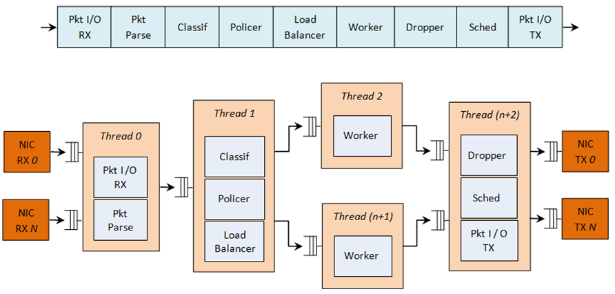
Fig. 23.2 Complex Packet Processing Pipeline with QoS Support
这个水线使用可重复使用的DPDK软件库构建。在这个流程中实现QoS的主要模块有:策略器,缓存器和调度器。下表列出了各块的功能描述。
| # | Block | Functional Description |
|---|---|---|
| 1 | Packet I/O RX & TX | 多个NIC端口的报文接收/传输。用于Intel 1GbE/10GbE NIC的轮询模式驱动程序(PMD)。 |
| 2 | Packet parser | 识别输入数据包的协议栈。检查数据包头部的完整性。 |
| 3 | Flow classification | 将输入数据包映射到已知流量上。 使用可配置散列函数(jhash,CRC等)和桶逻辑来处理冲突的精确匹配表查找。 |
| 4 | Policer | 使用srTCM(RFC 2697)或trTCM(RFC2698)算法进行数据包测量。 |
| 5 | Load Balancer | 将输入数据包分发给应用程序worker。为每个worker提供统一的负载。 保持流量对worker的亲和力和每个流程中的数据包顺序。 |
| 6 | Worker threads | 客户指定的应用工作负载的占位符(例如IP堆栈等)。 |
| 7 | Dropper | 拥塞管理使用随机早期检测(RED)算法(Sally Floyd-Van Jacobson的论文) 或加权RED(WRED)。根据当前调度程序队列的负载级别和报文优先级丢弃报文。 当遇到拥塞时,首先丢弃优先级较低的数据包。 |
| 8 | Hierarchical Scheduler | 具有数千(通常为64K)叶节点(队列)的5级分层调度器 (级别为:输出端口,子端口,管道,流量类和队列)。 实现流量整形(用于子站和管道级),严格优先级(对于流量级别) 和加权循环(WRR)(用于每个管道流量类中的队列)。 |
整个数据包处理流程中使用的基础架构块如下表所示。
| # | Block | Functional Description |
|---|---|---|
| 1 | Buffer manager | 支持全局缓冲池和专用的每线程缓存缓存。 |
| 2 | Queue manager | 支持水线之间的消息传递。 |
| 3 | Power saving | 在低活动期间支持节能。 |
水线块到CPU cores的映射可以根据每个特定应用程序所需的性能级别和为每个块启用的功能集进行配置。一些块可能会消耗多个CPU cores(每个CPU core在不同的输入数据包上运行同一个块的不同实例),而另外的几个块可以映射到同一个CPU core。
23.2. 分层调度
分层调度块(当存在时)通常位于发送阶段之前的TX侧。其目的是根据每个网络节点的服务级别协议(SLA)指定的策略来实现不同用户和不同流量类别的数据包传输。
23.2.1. 概述
分层调度类似于网络处理器使用的流量管理,通常实现每个流(或每组流)分组排队和调度。它像缓冲区一样工作,能够在传输之前临时存储大量数据包(入队操作);由于NIC TX正在请求更多的数据包进行传输,所以这些数据包随后被移出,并且随着分组选择逻辑观察预定义的SLA(出队操作)而交给NIC TX。
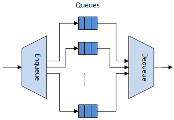
Fig. 23.3 Hierarchical Scheduler Block Internal Diagram
分层调度针对大量报文队列进行了优化。当只需要少量的队列时,应该使用消息传递队列而不是这个模块。有关更多详细的讨论,请参阅“Worst Case Scenarios for Performance”。
23.2.2. 调度层次
调度层次结构如下图所示。 Fig. 23.4. 层次结构的第一级是以太网TX端口1/10/40 GbE,后续层次级别定义为子端口,管道,流量类和队列。
通常,每个子端口表示预定义的用户组,而每个管道表示单个用户/订户。每个流量类是具有特定丢失率,延迟和抖动要求(例如语音,视频或数据传输)的不同流量类型的表示。每个队列都承载属于同一用户的同一类型的一个或多个连接的数据包。
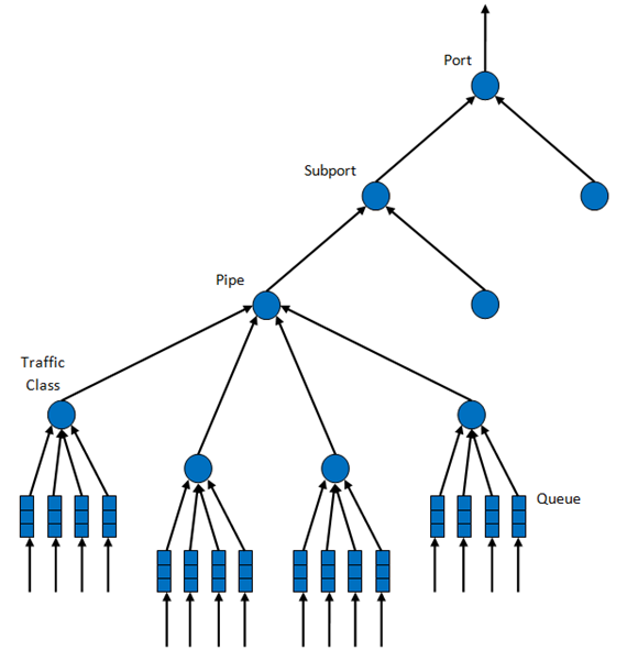
Fig. 23.4 Scheduling Hierarchy per Port
下表列出了各层次的功能。
| # | Level | Siblings per Parent | Functional Description |
|---|---|---|---|
| 1 | Port |
|
|
| 2 | Subport | Configurable (default: 8) |
|
| 3 | Pipe | Configurable (default: 4K) |
|
| 4 | Traffic Class (TC) | 4 |
|
| 5 | Queue | 4 |
|
23.2.3. 编程接口
23.2.3.1. PORT调度配置API
rte_sched.h文件包含port,subport和pipe的配置功能。
23.2.3.2. PORT调度入队API
Port调度入队API非常类似于DPDK PMD TX功能的API。
int rte_sched_port_enqueue(struct rte_sched_port *port, struct rte_mbuf **pkts, uint32_t n_pkts);
23.2.3.3. PORT调度出队API
Port调度入队API非常类似于DPDK PMD RX功能的API。
int rte_sched_port_dequeue(struct rte_sched_port *port, struct rte_mbuf **pkts, uint32_t n_pkts);
23.2.3.4. 用例
/* File "application.c" */

#define N_PKTS_RX   64
#define N_PKTS_TX   48
#define NIC_RX_PORT 0
#define NIC_RX_QUEUE 0
#define NIC_TX_PORT 1
#define NIC_TX_QUEUE 0

struct rte_sched_port *port = NULL;
struct rte_mbuf *pkts_rx[N_PKTS_RX], *pkts_tx[N_PKTS_TX];
uint32_t n_pkts_rx, n_pkts_tx;

/* Initialization */

<initialization code>

/* Runtime */
while (1) {
    /* Read packets from NIC RX queue */

    n_pkts_rx = rte_eth_rx_burst(NIC_RX_PORT, NIC_RX_QUEUE, pkts_rx, N_PKTS_RX);

    /* Hierarchical scheduler enqueue */

    rte_sched_port_enqueue(port, pkts_rx, n_pkts_rx);

    /* Hierarchical scheduler dequeue */

    n_pkts_tx = rte_sched_port_dequeue(port, pkts_tx, N_PKTS_TX);

    /* Write packets to NIC TX queue */

    rte_eth_tx_burst(NIC_TX_PORT, NIC_TX_QUEUE, pkts_tx, n_pkts_tx);
}
23.2.4. 实现
23.2.4.1. Internal Data Structures per Port
内部数据结构示意图,详细内容如下。
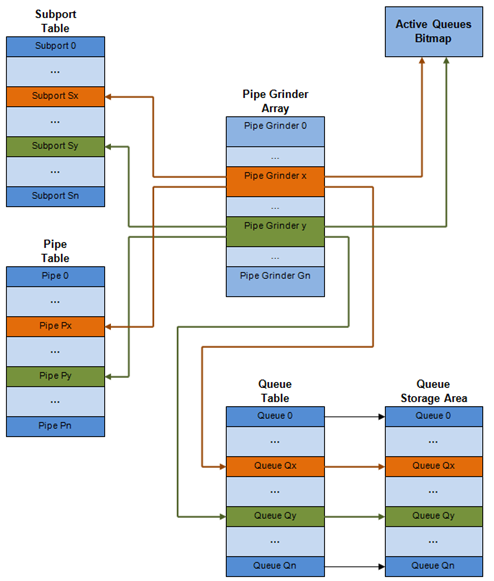
Fig. 23.5 Internal Data Structures per Port
| # | Data structure | Size (bytes) | # per port | Access type | Description | |
|---|---|---|---|---|---|---|
| Enq | Deq | |||||
| 1 | Subport table entry | 64 | # subports per port | Rd, Wr | 持续的子接口数据(信用,等) | |
| 2 | Pipe table entry | 64 | # pipes per port | Rd, Wr | 在运行时更新的pip,其TC及其队列的数据(信用等) pipe配置参数在运行时不改变。 相同的pipe配置参数由多个pipe共享, 因此它们不是pipe表条目的一部分。 |
|
| 3 | Queue table entry | 4 | #queues per port | Rd, Wr | Rd, Wr | 持续的队列数据(读写指针)。 对于所有队列,每个TC的队列大小相同, 允许使用快速公式计算队列基地址, 因此这两个参数不是队列表条目的一部分。 任何给定pipe的队列表条目都存储在同一个高速缓存行中 |
| 4 | Queue storage area | Config (default: 64 x8) | # queues per port | Wr | Rd | 每个队列的元素数组; 每个元素的大小是8字节mbuf指针 |
| 5 | Active queues bitmap | 1 bit per queue | 1 | Wr (Set) | Rd, Wr (Clear) | 位图为每个队列维护一个状态位: 队列不活动(队列为空)或队列活动(队列不为空) 队列位由调度程序入队设置,队列变空时清除。 位图扫描操作返回下一个非空pipe及其状态 (pipe中活动队列的16位掩码)。 |
| 6 | Grinder | ~128 | Config (default: 8) | Rd, Wr | 目前正在处理的活动pipe列表。 grinder在pipe加工过程中包含临时数据。 一旦当前pipe排出数据包或信用点, 它将从位图中的另一个活动管道替换。 |
|
23.2.4.2. 多核缩放策略
多核缩放策略如下:
- 在不同线程上操作不同的物理端口。但是同一个端口的入队和出队由同一个线程执行。
- 通过在不同线程上操作相同物理端口(虚拟端口)的不同组的子端口,可以将相同的物理端口拆分到不同的线程。类似地,子端口可以被分割成更多个子端口,每个子端口由不同的线程运行。但是同一个端口的入队和出队由同一个线程运行。仅当出于性能考虑,不可能使用单个core处理完整端口时,才这样处理。
23.2.4.2.1. 同一输出端口的出队和入队
上面强调过,同一个端口的出队和入队需要由同一个线程执行。因为,在不同core上对同一个输出端口执行出队和入队操作,可能会对调度程序的性能造成重大影响,因此不推荐这样做。
同一端口的入队和出队操作共享以下数据结构的访问权限:
- 报文描述符
- 队列表
- 队列存储空区
- 活动队列位图
可能存在使性能下降的原因如下:
- 需要使队列和位图操作线程安全,这可能需要使用锁以保证访问顺序(例如,自旋锁/信号量)或使用原子操作进行无锁访问(例如,Test and Set或Compare and Swap命令等))。前一种情况对性能影响要严重得多。
- 在两个core之间对存储共享数据结构的缓存行执行乒乓操作(由MESI协议缓存一致性CPU硬件透明地完成)。
当调度程序入队和出队操作必须在同一个线程运行,允许队列和位图操作非线程安全,并将调度程序数据结构保持在同一个core上,可以很大程度上保证性能。
23.2.4.2.2. 性能缩放
扩展NIC端口数量只需要保证用于流量调度的CPU内核数量按比例增加即可。
23.2.4.3. 入队水线
每个数据包的入队步骤:
- 访问mbuf以读取标识数据包的目标队列所需的字段。这些字段包括port,subport,traffic class及queue,并且通常由报文分类阶段设置。
- 访问队列结构以识别队列数组中的写入位置。如果队列已满,则丢弃该数据包。
- 访问队列阵列位置以存储数据包(即写入mbuf指针)。
应该注意到这些步骤之间具有很强的数据依赖性,因为步骤2和3在步骤1和2的结果变得可用之前无法启动,这样就无法使用处理器乱序执行引擎上提供任何显着的性能优化。
考虑这样一种情况,给定的输入报文速率很高,队列数量大,可以想象得到,入队当前数据包需要访问的数据结构不存在于当前core的L1或L2 data cache中,此时,上述3个内存访问操作将会产生L1和L2 data cache miss。就性能考虑而言,每个数据包出现3次L1 / L2 data cache miss是不可接受的。
解决方法是提前预取所需的数据结构。预取操作具有执行延迟,在此期间处理器不应尝试访问当前正在进行预取的数据结构,此时处理器转向执行其他工作。可用的其他工作可以是对其他输入报文执行不同阶段的入队序列,从而实现入队操作的流水线实现。
Fig. 23.6 展示出了具有4级水线的入队操作实现,并且每个阶段操作2个不同的输入报文。在给定的时间点上,任何报文只能在水线某个阶段进行处理。
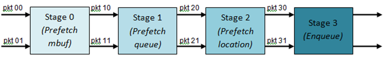
Fig. 23.6 Prefetch Pipeline for the Hierarchical Scheduler Enqueue Operation
由上图描述的入队水线实现的拥塞管理方案是非常基础的:数据包排队入队,直到指定队列变满为止;当满时,到这个队列的所有数据包将被丢弃,直到队列中有数据包出队。可以通过使用RED/WRED作为入队水线的一部分来改进,该流程查看队列占用率和报文优先级,以便产生特定数据包的入队/丢弃决定(与入队所有数据包/不加区分地丢弃所有数据包不一样)。
23.2.4.4. 出队状态机
从当前pipe调度下一个数据包的步骤如下:
- 使用位图扫描操作识别出下一个活动的pipe(prefetch pipe)。
- 读取pipe数据结构。更新当前pipe及其subport的信用。识别当前pipe中的第一个active traffic class,使用WRR选择下一个queue,为当前pipe的所有16个queue预取队列指针。
- 从当前WRR queue读取下一个元素,并预取其数据包描述符。
- 从包描述符(mbuf结构)读取包长度。根据包长度和可用信用(当前pipe,pipe traffic class,subport及subport traffic class),对当前数据包进行是否调度决策。
为了避免cache miss,上述数据结构(pipe,queue,queue array,mbufs)在被访问之前被预取。隐藏预取操作的延迟的策略是在为当前pipe发出预取后立即从当前pipe(在grinder A中)切换到另一个pipe(在grinderB中)。这样就可以在执行切换回pipe(grinder A)之前,有足够的时间完成预取操作。
出pipe状态机将数据存在处理器高速缓存中,因此它尝试从相同的pipe TC和pipe(尽可能多的数据包和信用)发送尽可能多的数据包,然后再移动到下一个活动TC pipe(如果有)或另一个活动pipe。 .. _figure_pipe_prefetch_sm:
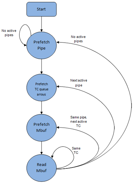
Fig. 23.7 Pipe Prefetch State Machine for the Hierarchical Scheduler Dequeue Operation
23.2.4.5. 时间和同步
输出端口被建模为字节槽的传送带,需要由调度器填充用于传输的数据。对于10GbE,每秒需要由调度器填充12.5亿个字节的槽位。如果调度程序填充不够快,只要存在足够的报文和信用,则一些时隙将被闲置并且带宽将被浪费。
原则上,层次调度程序出队操作应由NIC TX触发。通常,一旦NIC TX输入队列的占用率下降到预定义的阈值以下,端口调度器将被唤醒(基于中断或基于轮询,通过连续监视队列占用)来填充更多的数据包进入队列。
23.2.4.5.1. 内部时间引用
调度器需要跟踪信用逻辑的时间演化,因为信用需要基于时间更新(例如,子流量和管道流量整形,流量级上限执行等)。
每当调度程序决定将数据包发送到NIC TX进行传输时,调度器将相应地增加其内部时间参考。因此,以字节为单位保持内部时间基准是方便的,其中字节表示物理接口在传输介质上发送字节所需的持续时间。这样,当报文被调度用于传输时,时间以(n + h)递增,其中n是以字节为单位的报文长度,h是每个报文的成帧开销字节数。
23.2.4.5.2. 内部时间参考重新同步
调度器需要将其内部时间参考对齐到端口传送带的步速。原因是要确保调度程序不以比物理介质的线路速率更多的字节来馈送NIC TX,以防止数据包丢失。
调度程序读取每个出队调用的当前时间。可以通过读取时间戳计数器(TSC)寄存器或高精度事件定时器(HPET)寄存器来获取CPU时间戳。 当前CPU时间戳将CPU时钟数转换为字节数:time_bytes = time_cycles / cycles_per_byte,其中cycles_per_byte是等效于线上一个字节的传输时间的CPU周期数(例如CPU频率 2 GHz和10GbE端口, cycles_per_byte = 1.6 )。
调度程序维护NIC time的内部时间参考。 每当分组被调度时,NIC time随分组长度(包括帧开销)增加。在每次出队调用时,调度程序将检查其NIC time的内部引用与当前时间的关系:
- 如果NIC time未来(NIC time> =当前时间),则不需要调整NIC time。这意味着调度程序能够在NIC实际需要这些数据包之前安排NIC数据包,因此NIC TX提供了数据包;
- 如果NIC time过去(NIC时间<当前时间),则NIC time应通过将其设置为当前时间来进行调整。 这意味着调度程序不能跟上NIC字节传送带的速度,因此由于NIC TX的数据包供应不足,所以NIC带宽被浪费了。
23.2.4.5.3. 调度器精度和粒度
调度器往返延迟(SRTD)是指调度器在同一个pipe的两次连续检验之间的时间(CPU周期数)。
为了跟上输出端口(即避免带宽丢失),调度程序应该能够比NIC TX发送的n个数据包更快地调度n个数据包。
假设没有端口超过流量,调度程序需要跟上管道令牌桶配置的每个管道的速率。这意味着管道令牌桶的大小应该设置得足够高,以防止它由于大的SRTD而溢出,因为这将导致管道的信用损失(带宽损失)。
23.2.4.6. 信用逻辑
23.2.4.6.1. 调度决策
当满足以下所有条件时,从(subport S,pipe P,traffic class TC,queue Q)发送下一个分组的调度决定(分组被发送):
- Subport S的Pipe P目前由一个端口调度选择;
- 流量类TC是管道P的最高优先级的主要流量类别;
- 队列Q是管道P的流量类TC内由WRR选择的下一个队列;
- 子接口S有足够的信用来发送数据包;
- 子接口S具有足够的信用流量类TC来发送数据包;
- 管道P有足够的信用来发送数据包;
- 管道P具有足够的信用用于流量类TC发送数据包。
如果满足所有上述条件,则选择分组进行传输,并从子接口S,子接口S流量类TC,管道P,管道P流量类TC中减去必要的信用。
23.2.4.6.2. 帧开销
由于所有数据包长度的最大公约数为1个字节,所以信用单位被选为1个字节。传输n个字节的报文所需的信用数量等于(n + h),其中h等于每个报文的成帧开销字节数。
| # | Packet field | Length (bytes) | Comments |
|---|---|---|---|
| 1 | Preamble | 7 | |
| 2 | Start of Frame Delimiter (SFD) | 1 | |
| 3 | Frame Check Sequence (FCS) | 4 | 当mbuf包长度字段中不包含时这里才需要考虑开销。 |
| 4 | Inter Frame Gap (IFG) | 12 | |
| 5 | Total | 24 |
23.2.4.6.3. Traffic Shaping
The traffic shaping for subport and pipe is implemented using a token bucket per subport/per pipe. Each token bucket is implemented using one saturated counter that keeps track of the number of available credits.
The token bucket generic parameters and operations are presented in Table 23.6 and Table 23.7.
| # | Token Bucket Parameter | Unit | Description |
|---|---|---|---|
| 1 | bucket_rate | Credits per second | Rate of adding credits to the bucket. |
| 2 | bucket_size | Credits | Max number of credits that can be stored in the bucket. |
| # | Token Bucket Operation | Description |
|---|---|---|
| 1 | Initialization | Bucket set to a predefined value, e.g. zero or half of the bucket size. |
| 2 | Credit update | Credits are added to the bucket on top of existing ones, either periodically or on demand, based on the bucket_rate. Credits cannot exceed the upper limit defined by the bucket_size, so any credits to be added to the bucket while the bucket is full are dropped. |
| 3 | Credit consumption | As result of packet scheduling, the necessary number of credits is removed from the bucket. The packet can only be sent if enough credits are in the bucket to send the full packet (packet bytes and framing overhead for the packet). |
To implement the token bucket generic operations described above, the current design uses the persistent data structure presented in Table 23.8, while the implementation of the token bucket operations is described in Table 23.9.
| # | Token bucket field | Unit | Description |
|---|---|---|---|
| 1 | tb_time | Bytes | Time of the last credit update. Measured in bytes instead of seconds or CPU cycles for ease of credit consumption operation (as the current time is also maintained in bytes). See Section 26.2.4.5.1 “Internal Time Reference” for an explanation of why the time is maintained in byte units. |
| 2 | tb_period | Bytes | Time period that should elapse since the last credit update in order for the bucket to be awarded tb_credits_per_period worth or credits. |
| 3 | tb_credits_per_period | Bytes | Credit allowance per tb_period. |
| 4 | tb_size | Bytes | Bucket size, i.e. upper limit for the tb_credits. |
| 5 | tb_credits | Bytes | Number of credits currently in the bucket. |
The bucket rate (in bytes per second) can be computed with the following formula:
bucket_rate = (tb_credits_per_period / tb_period) * r
where, r = port line rate (in bytes per second).
| # | Token bucket operation | Description |
|---|---|---|
| 1 | Initialization | tb_credits = 0; or tb_credits = tb_size / 2; |
| 2 | Credit update | Credit update options:
The current implementation is using option 3. According to Section “Dequeue State Machine”, the pipe and subport credits are updated every time a pipe is selected by the dequeue process before the pipe and subport credits are actually used. The implementation uses a tradeoff between accuracy and speed by updating the bucket credits only when at least a full tb_period has elapsed since the last update.
Update operations:
|
| 3 |
|
As result of packet scheduling, the necessary number of credits is removed from the bucket. The packet can only be sent if enough credits are in the bucket to send the full packet (packet bytes and framing overhead for the packet). Scheduling operations: pkt_credits = pkt_len + frame_overhead; if (tb_credits >= pkt_credits){tb_credits -= pkt_credits;} |
23.2.4.6.4. Traffic Classes
23.2.4.6.4.1. Implementation of Strict Priority Scheduling
Strict priority scheduling of traffic classes within the same pipe is implemented by the pipe dequeue state machine, which selects the queues in ascending order. Therefore, queues 0..3 (associated with TC 0, highest priority TC) are handled before queues 4..7 (TC 1, lower priority than TC 0), which are handled before queues 8..11 (TC 2), which are handled before queues 12..15 (TC 3, lowest priority TC).
23.2.4.6.4.2. Upper Limit Enforcement
The traffic classes at the pipe and subport levels are not traffic shaped, so there is no token bucket maintained in this context. The upper limit for the traffic classes at the subport and pipe levels is enforced by periodically refilling the subport / pipe traffic class credit counter, out of which credits are consumed every time a packet is scheduled for that subport / pipe, as described in Table 23.10 and Table 23.11.
| # | Subport or pipe field | Unit | Description |
|---|---|---|---|
| 1 | tc_time | Bytes | Time of the next update (upper limit refill) for the 4 TCs of the current subport / pipe. See Section “Internal Time Reference”for the explanation of why the time is maintained in byte units. |
| 2 | tc_period | Bytes | Time between two consecutive updates for the 4 TCs of the current subport / pipe. This is expected to be many times bigger than the typical value of the token bucket tb_period. |
| 3 | tc_credits_per_period | Bytes | Upper limit for the number of credits allowed to be consumed by the current TC during each enforcement period tc_period. |
| 4 | tc_credits | Bytes | Current upper limit for the number of credits that can be consumed by the current traffic class for the remainder of the current enforcement period. |
| # | Traffic Class Operation | Description |
|---|---|---|
| 1 | Initialization | tc_credits = tc_credits_per_period; tc_time = tc_period; |
| 2 | Credit update | Update operations: if (time >= tc_time) { tc_credits = tc_credits_per_period; tc_time = time + tc_period; } |
| 3 | Credit consumption (on packet scheduling) | As result of packet scheduling, the TC limit is decreased with the necessary number of credits. The packet can only be sent if enough credits are currently available in the TC limit to send the full packet (packet bytes and framing overhead for the packet). Scheduling operations: pkt_credits = pk_len + frame_overhead; if (tc_credits >= pkt_credits) {tc_credits -= pkt_credits;} |
23.2.4.6.5. Weighted Round Robin (WRR)
The evolution of the WRR design solution from simple to complex is shown in Table 23.12.
| # | All Queues Active? | Equal Weights for All Queues? | All Packets Equal? | Strategy |
|---|---|---|---|---|
| 1 | Yes | Yes | Yes | Byte level round robin Next queue queue #i, i = (i + 1) % n |
| 2 | Yes | Yes | No | Packet level round robin Consuming one byte from queue #i requires consuming exactly one token for queue #i. T(i) = Accumulated number of tokens previously consumed from queue #i. Every time a packet is consumed from queue #i, T(i) is updated as: T(i) += pkt_len. Next queue : queue with the smallest T. |
| 3 | Yes | No | No | Packet level weighted round robin This case can be reduced to the previous case by introducing a cost per byte that is different for each queue. Queues with lower weights have a higher cost per byte. This way, it is still meaningful to compare the consumption amongst different queues in order to select the next queue. w(i) = Weight of queue #i t(i) = Tokens per byte for queue #i, defined as the inverse weight of queue #i. For example, if w[0..3] = [1:2:4:8], then t[0..3] = [8:4:2:1]; if w[0..3] = [1:4:15:20], then t[0..3] = [60:15:4:3]. Consuming one byte from queue #i requires consuming t(i) tokens for queue #i. T(i) = Accumulated number of tokens previously consumed from queue #i. Every time a packet is consumed from queue #i, T(i) is updated as: T(i) += pkt_len * t(i). Next queue : queue with the smallest T. |
| 4 | No | No | No | Packet level weighted round robin with variable queue status Reduce this case to the previous case by setting the consumption of inactive queues to a high number, so that the inactive queues will never be selected by the smallest T logic. To prevent T from overflowing as result of successive accumulations, T(i) is truncated after each packet consumption for all queues. For example, T[0..3] = [1000, 1100, 1200, 1300] is truncated to T[0..3] = [0, 100, 200, 300] by subtracting the min T from T(i), i = 0..n. This requires having at least one active queue in the set of input queues, which is guaranteed by the dequeue state machine never selecting an inactive traffic class. mask(i) = Saturation mask for queue #i, defined as: mask(i) = (queue #i is active)? 0 : 0xFFFFFFFF; w(i) = Weight of queue #i t(i) = Tokens per byte for queue #i, defined as the inverse weight of queue #i. T(i) = Accumulated numbers of tokens previously consumed from queue #i. Next queue : queue with smallest T. Before packet consumption from queue #i: T(i) |= mask(i) After packet consumption from queue #i: T(j) -= T(i), j != i T(i) = pkt_len * t(i) Note: T(j) uses the T(i) value before T(i) is updated. |
23.2.4.6.6. Subport Traffic Class Oversubscription
23.2.4.6.6.1. Problem Statement
Oversubscription for subport traffic class X is a configuration-time event that occurs when more bandwidth is allocated for traffic class X at the level of subport member pipes than allocated for the same traffic class at the parent subport level.
The existence of the oversubscription for a specific subport and traffic class is solely the result of pipe and subport-level configuration as opposed to being created due to dynamic evolution of the traffic load at run-time (as congestion is).
When the overall demand for traffic class X for the current subport is low, the existence of the oversubscription condition does not represent a problem, as demand for traffic class X is completely satisfied for all member pipes. However, this can no longer be achieved when the aggregated demand for traffic class X for all subport member pipes exceeds the limit configured at the subport level.
23.2.4.6.6.2. Solution Space
summarizes some of the possible approaches for handling this problem, with the third approach selected for implementation.
| No. | Approach | Description |
|---|---|---|
| 1 | Don’t care | First come, first served. This approach is not fair amongst subport member pipes, as pipes that are served first will use up as much bandwidth for TC X as they need, while pipes that are served later will receive poor service due to bandwidth for TC X at the subport level being scarce. |
| 2 | Scale down all pipes | All pipes within the subport have their bandwidth limit for TC X scaled down by the same factor. This approach is not fair among subport member pipes, as the low end pipes (that is, pipes configured with low bandwidth) can potentially experience severe service degradation that might render their service unusable (if available bandwidth for these pipes drops below the minimum requirements for a workable service), while the service degradation for high end pipes might not be noticeable at all. |
| 3 | Cap the high demand pipes | Each subport member pipe receives an equal share of the bandwidth available at run-time for TC X at the subport level. Any bandwidth left unused by the low-demand pipes is redistributed in equal portions to the high-demand pipes. This way, the high-demand pipes are truncated while the low-demand pipes are not impacted. |
Typically, the subport TC oversubscription feature is enabled only for the lowest priority traffic class (TC 3), which is typically used for best effort traffic, with the management plane preventing this condition from occurring for the other (higher priority) traffic classes.
To ease implementation, it is also assumed that the upper limit for subport TC 3 is set to 100% of the subport rate, and that the upper limit for pipe TC 3 is set to 100% of pipe rate for all subport member pipes.
23.2.4.6.6.3. Implementation Overview
The algorithm computes a watermark, which is periodically updated based on the current demand experienced by the subport member pipes, whose purpose is to limit the amount of traffic that each pipe is allowed to send for TC 3. The watermark is computed at the subport level at the beginning of each traffic class upper limit enforcement period and the same value is used by all the subport member pipes throughout the current enforcement period. illustrates how the watermark computed as subport level at the beginning of each period is propagated to all subport member pipes.
At the beginning of the current enforcement period (which coincides with the end of the previous enforcement period), the value of the watermark is adjusted based on the amount of bandwidth allocated to TC 3 at the beginning of the previous period that was not left unused by the subport member pipes at the end of the previous period.
If there was subport TC 3 bandwidth left unused, the value of the watermark for the current period is increased to encourage the subport member pipes to consume more bandwidth. Otherwise, the value of the watermark is decreased to enforce equality of bandwidth consumption among subport member pipes for TC 3.
The increase or decrease in the watermark value is done in small increments, so several enforcement periods might be required to reach the equilibrium state. This state can change at any moment due to variations in the demand experienced by the subport member pipes for TC 3, for example, as a result of demand increase (when the watermark needs to be lowered) or demand decrease (when the watermark needs to be increased).
When demand is low, the watermark is set high to prevent it from impeding the subport member pipes from consuming more bandwidth. The highest value for the watermark is picked as the highest rate configured for a subport member pipe. Table 23.14 and Table 23.15 illustrates the watermark operation.
| No. | Subport Traffic Class Operation | Description |
|---|---|---|
| 1 | Initialization | Subport level: subport_period_id= 0 Pipe level: pipe_period_id = 0 |
| 2 | Credit update | Subport Level: if (time>=subport_tc_time)
} Pipelevel: if(pipe_period_id != subport_period_id) {
} |
| 3 | Credit consumption (on packet scheduling) | Pipe level: pkt_credits = pk_len + frame_overhead; if(pipe_ov_credits >= pkt_credits{
} |
| No. | Subport Traffic Class Operation | Description |
|---|---|---|
| 1 | Initialization | Subport level: wm = WM_MAX |
| 2 | Credit update | Subport level (water_mark_update): tc0_cons = subport_tc0_credits_per_period - subport_tc0_credits; tc1_cons = subport_tc1_credits_per_period - subport_tc1_credits; tc2_cons = subport_tc2_credits_per_period - subport_tc2_credits; tc3_cons = subport_tc3_credits_per_period - subport_tc3_credits; tc3_cons_max = subport_tc3_credits_per_period - (tc0_cons + tc1_cons + tc2_cons); if(tc3_consumption > (tc3_consumption_max - MTU)){
} else {
} |
23.2.5. Worst Case Scenarios for Performance
23.2.5.1. Lots of Active Queues with Not Enough Credits
The more queues the scheduler has to examine for packets and credits in order to select one packet, the lower the performance of the scheduler is.
The scheduler maintains the bitmap of active queues, which skips the non-active queues, but in order to detect whether a specific pipe has enough credits, the pipe has to be drilled down using the pipe dequeue state machine, which consumes cycles regardless of the scheduling result (no packets are produced or at least one packet is produced).
This scenario stresses the importance of the policer for the scheduler performance: if the pipe does not have enough credits, its packets should be dropped as soon as possible (before they reach the hierarchical scheduler), thus rendering the pipe queues as not active, which allows the dequeue side to skip that pipe with no cycles being spent on investigating the pipe credits that would result in a “not enough credits” status.
23.2.5.2. Single Queue with 100% Line Rate
The port scheduler performance is optimized for a large number of queues. If the number of queues is small, then the performance of the port scheduler for the same level of active traffic is expected to be worse than the performance of a small set of message passing queues.
23.3. Dropper
The purpose of the DPDK dropper is to drop packets arriving at a packet scheduler to avoid congestion. The dropper supports the Random Early Detection (RED), Weighted Random Early Detection (WRED) and tail drop algorithms. Fig. 23.8 illustrates how the dropper integrates with the scheduler. The DPDK currently does not support congestion management so the dropper provides the only method for congestion avoidance.
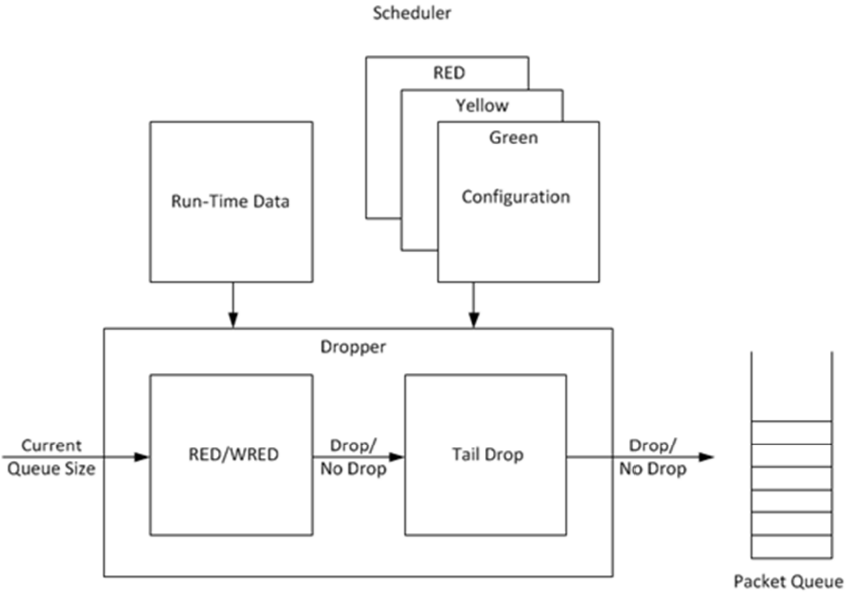
Fig. 23.8 High-level Block Diagram of the DPDK Dropper
The dropper uses the Random Early Detection (RED) congestion avoidance algorithm as documented in the reference publication. The purpose of the RED algorithm is to monitor a packet queue, determine the current congestion level in the queue and decide whether an arriving packet should be enqueued or dropped. The RED algorithm uses an Exponential Weighted Moving Average (EWMA) filter to compute average queue size which gives an indication of the current congestion level in the queue.
For each enqueue operation, the RED algorithm compares the average queue size to minimum and maximum thresholds. Depending on whether the average queue size is below, above or in between these thresholds, the RED algorithm calculates the probability that an arriving packet should be dropped and makes a random decision based on this probability.
The dropper also supports Weighted Random Early Detection (WRED) by allowing the scheduler to select different RED configurations for the same packet queue at run-time. In the case of severe congestion, the dropper resorts to tail drop. This occurs when a packet queue has reached maximum capacity and cannot store any more packets. In this situation, all arriving packets are dropped.
The flow through the dropper is illustrated in Fig. 23.9. The RED/WRED algorithm is exercised first and tail drop second.
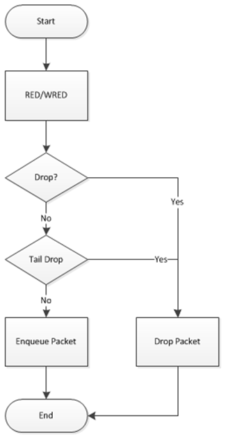
Fig. 23.9 Flow Through the Dropper
The use cases supported by the dropper are:
- Initialize configuration data
- Initialize run-time data
- Enqueue (make a decision to enqueue or drop an arriving packet)
- Mark empty (record the time at which a packet queue becomes empty)
The configuration use case is explained in Section2.23.3.1, the enqueue operation is explained in Section 2.23.3.2 and the mark empty operation is explained in Section 2.23.3.3.
23.3.1. Configuration
A RED configuration contains the parameters given in Table 23.16.
| Parameter | Minimum | Maximum | Typical |
|---|---|---|---|
| Minimum Threshold | 0 | 1022 | 1/4 x queue size |
| Maximum Threshold | 1 | 1023 | 1/2 x queue size |
| Inverse Mark Probability | 1 | 255 | 10 |
| EWMA Filter Weight | 1 | 12 | 9 |
The meaning of these parameters is explained in more detail in the following sections. The format of these parameters as specified to the dropper module API corresponds to the format used by Cisco* in their RED implementation. The minimum and maximum threshold parameters are specified to the dropper module in terms of number of packets. The mark probability parameter is specified as an inverse value, for example, an inverse mark probability parameter value of 10 corresponds to a mark probability of 1/10 (that is, 1 in 10 packets will be dropped). The EWMA filter weight parameter is specified as an inverse log value, for example, a filter weight parameter value of 9 corresponds to a filter weight of 1/29.
23.3.2. Enqueue Operation
In the example shown in Fig. 23.10, q (actual queue size) is the input value, avg (average queue size) and count (number of packets since the last drop) are run-time values, decision is the output value and the remaining values are configuration parameters.
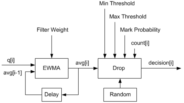
Fig. 23.10 Example Data Flow Through Dropper
23.3.2.1. EWMA Filter Microblock
The purpose of the EWMA Filter microblock is to filter queue size values to smooth out transient changes that result from “bursty” traffic. The output value is the average queue size which gives a more stable view of the current congestion level in the queue.
The EWMA filter has one configuration parameter, filter weight, which determines how quickly or slowly the average queue size output responds to changes in the actual queue size input. Higher values of filter weight mean that the average queue size responds more quickly to changes in actual queue size.
23.3.2.1.1. Average Queue Size Calculation when the Queue is not Empty
The definition of the EWMA filter is given in the following equation.
Where:
- avg = average queue size
- wq = filter weight
- q = actual queue size
Note
- The filter weight, wq = 1/2^n, where n is the filter weight parameter value passed to the dropper module
- on configuration (see Section2.23.3.1 ).
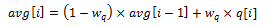
23.3.2.2. Average Queue Size Calculation when the Queue is Empty
The EWMA filter does not read time stamps and instead assumes that enqueue operations will happen quite regularly. Special handling is required when the queue becomes empty as the queue could be empty for a short time or a long time. When the queue becomes empty, average queue size should decay gradually to zero instead of dropping suddenly to zero or remaining stagnant at the last computed value. When a packet is enqueued on an empty queue, the average queue size is computed using the following formula:
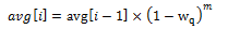
Where:
- m = the number of enqueue operations that could have occurred on this queue while the queue was empty
In the dropper module, m is defined as:
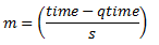
Where:
- time = current time
- qtime = time the queue became empty
- s = typical time between successive enqueue operations on this queue
The time reference is in units of bytes, where a byte signifies the time duration required by the physical interface to send out a byte on the transmission medium (see Section “Internal Time Reference”). The parameter s is defined in the dropper module as a constant with the value: s=2^22. This corresponds to the time required by every leaf node in a hierarchy with 64K leaf nodes to transmit one 64-byte packet onto the wire and represents the worst case scenario. For much smaller scheduler hierarchies, it may be necessary to reduce the parameter s, which is defined in the red header source file (rte_red.h) as:
#define RTE_RED_S
Since the time reference is in bytes, the port speed is implied in the expression: time-qtime. The dropper does not have to be configured with the actual port speed. It adjusts automatically to low speed and high speed links.
23.3.2.2.1. Implementation
A numerical method is used to compute the factor (1-wq)^m that appears in Equation 2.
This method is based on the following identity:
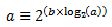
This allows us to express the following:
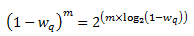
In the dropper module, a look-up table is used to compute log2(1-wq) for each value of wq supported by the dropper module. The factor (1-wq)^m can then be obtained by multiplying the table value by m and applying shift operations. To avoid overflow in the multiplication, the value, m, and the look-up table values are limited to 16 bits. The total size of the look-up table is 56 bytes. Once the factor (1-wq)^m is obtained using this method, the average queue size can be calculated from Equation 2.
23.3.2.2.2. Alternative Approaches
Other methods for calculating the factor (1-wq)^m in the expression for computing average queue size when the queue is empty (Equation 2) were considered. These approaches include:
- Floating-point evaluation
- Fixed-point evaluation using a small look-up table (512B) and up to 16 multiplications (this is the approach used in the FreeBSD* ALTQ RED implementation)
- Fixed-point evaluation using a small look-up table (512B) and 16 SSE multiplications (SSE optimized version of the approach used in the FreeBSD* ALTQ RED implementation)
- Large look-up table (76 KB)
The method that was finally selected (described above in Section 26.3.2.2.1) out performs all of these approaches in terms of run-time performance and memory requirements and also achieves accuracy comparable to floating-point evaluation. Table 23.17 lists the performance of each of these alternative approaches relative to the method that is used in the dropper. As can be seen, the floating-point implementation achieved the worst performance.
| Method | Relative Performance |
|---|---|
| Current dropper method (see Section 23.3.2.1.3) | 100% |
| Fixed-point method with small (512B) look-up table | 148% |
| SSE method with small (512B) look-up table | 114% |
| Large (76KB) look-up table | 118% |
| Floating-point | 595% |
| Note: In this case, since performance is expressed as time spent executing the operation in a specific condition, any relative performance value above 100% runs slower than the reference method. | |
23.3.2.3. Drop Decision Block
The Drop Decision block:
- Compares the average queue size with the minimum and maximum thresholds
- Calculates a packet drop probability
- Makes a random decision to enqueue or drop an arriving packet
The calculation of the drop probability occurs in two stages. An initial drop probability is calculated based on the average queue size, the minimum and maximum thresholds and the mark probability. An actual drop probability is then computed from the initial drop probability. The actual drop probability takes the count run-time value into consideration so that the actual drop probability increases as more packets arrive to the packet queue since the last packet was dropped.
23.3.2.3.1. Initial Packet Drop Probability
The initial drop probability is calculated using the following equation.
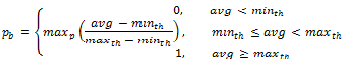
Where:
- maxp = mark probability
- avg = average queue size
- minth = minimum threshold
- maxth = maximum threshold
The calculation of the packet drop probability using Equation 3 is illustrated in Fig. 23.11. If the average queue size is below the minimum threshold, an arriving packet is enqueued. If the average queue size is at or above the maximum threshold, an arriving packet is dropped. If the average queue size is between the minimum and maximum thresholds, a drop probability is calculated to determine if the packet should be enqueued or dropped.
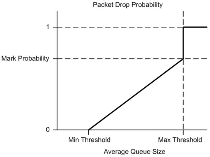
Fig. 23.11 Packet Drop Probability for a Given RED Configuration
23.3.2.3.2. Actual Drop Probability
If the average queue size is between the minimum and maximum thresholds, then the actual drop probability is calculated from the following equation.
Where:
- Pb = initial drop probability (from Equation 3)
- count = number of packets that have arrived since the last drop
The constant 2, in Equation 4 is the only deviation from the drop probability formulae given in the reference document where a value of 1 is used instead. It should be noted that the value pa computed from can be negative or greater than 1. If this is the case, then a value of 1 should be used instead.
The initial and actual drop probabilities are shown in Fig. 23.12. The actual drop probability is shown for the case where the formula given in the reference document1 is used (blue curve) and also for the case where the formula implemented in the dropper module, is used (red curve). The formula in the reference document results in a significantly higher drop rate compared to the mark probability configuration parameter specified by the user. The choice to deviate from the reference document is simply a design decision and one that has been taken by other RED implementations, for example, FreeBSD* ALTQ RED.
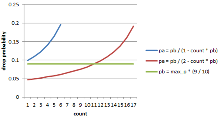
Fig. 23.12 Initial Drop Probability (pb), Actual Drop probability (pa) Computed Using a Factor 1 (Blue Curve) and a Factor 2 (Red Curve)
23.3.3. Queue Empty Operation
The time at which a packet queue becomes empty must be recorded and saved with the RED run-time data so that the EWMA filter block can calculate the average queue size on the next enqueue operation. It is the responsibility of the calling application to inform the dropper module through the API that a queue has become empty.
23.3.4. Source Files Location
The source files for the DPDK dropper are located at:
- DPDK/lib/librte_sched/rte_red.h
- DPDK/lib/librte_sched/rte_red.c
23.3.5. Integration with the DPDK QoS Scheduler
RED functionality in the DPDK QoS scheduler is disabled by default. To enable it, use the DPDK configuration parameter:
CONFIG_RTE_SCHED_RED=y
This parameter must be set to y. The parameter is found in the build configuration files in the DPDK/config directory, for example, DPDK/config/common_linuxapp. RED configuration parameters are specified in the rte_red_params structure within the rte_sched_port_params structure that is passed to the scheduler on initialization. RED parameters are specified separately for four traffic classes and three packet colors (green, yellow and red) allowing the scheduler to implement Weighted Random Early Detection (WRED).
23.3.6. Integration with the DPDK QoS Scheduler Sample Application
The DPDK QoS Scheduler Application reads a configuration file on start-up. The configuration file includes a section containing RED parameters. The format of these parameters is described in Section2.23.3.1. A sample RED configuration is shown below. In this example, the queue size is 64 packets.
Note
For correct operation, the same EWMA filter weight parameter (wred weight) should be used for each packet color (green, yellow, red) in the same traffic class (tc).
 ; RED params per traffic class and color (Green / Yellow / Red)

[red]
tc 0 wred min = 28 22 16
tc 0 wred max = 32 32 32
tc 0 wred inv prob = 10 10 10
tc 0 wred weight = 9 9 9

tc 1 wred min = 28 22 16
tc 1 wred max = 32 32 32
tc 1 wred inv prob = 10 10 10
tc 1 wred weight = 9 9 9

tc 2 wred min = 28 22 16
tc 2 wred max = 32 32 32
tc 2 wred inv prob = 10 10 10
tc 2 wred weight = 9 9 9

tc 3 wred min = 28 22 16
tc 3 wred max = 32 32 32
tc 3 wred inv prob = 10 10 10
tc 3 wred weight = 9 9 9
With this configuration file, the RED configuration that applies to green, yellow and red packets in traffic class 0 is shown in Table 23.18.
| RED Parameter | Configuration Name | Green | Yellow | Red |
|---|---|---|---|---|
| Minimum Threshold | tc 0 wred min | 28 | 22 | 16 |
| Maximum Threshold | tc 0 wred max | 32 | 32 | 32 |
| Mark Probability | tc 0 wred inv prob | 10 | 10 | 10 |
| EWMA Filter Weight | tc 0 wred weight | 9 | 9 | 9 |
23.3.7. Application Programming Interface (API)
23.3.7.1. Enqueue API
The syntax of the enqueue API is as follows:
int rte_red_enqueue(const struct rte_red_config *red_cfg, struct rte_red *red, const unsigned q, const uint64_t time)
The arguments passed to the enqueue API are configuration data, run-time data, the current size of the packet queue (in packets) and a value representing the current time. The time reference is in units of bytes, where a byte signifies the time duration required by the physical interface to send out a byte on the transmission medium (see Section 26.2.4.5.1 “Internal Time Reference” ). The dropper reuses the scheduler time stamps for performance reasons.
23.3.7.2. Empty API
The syntax of the empty API is as follows:
void rte_red_mark_queue_empty(struct rte_red *red, const uint64_t time)
The arguments passed to the empty API are run-time data and the current time in bytes.
23.4. Traffic Metering
The traffic metering component implements the Single Rate Three Color Marker (srTCM) and Two Rate Three Color Marker (trTCM) algorithms, as defined by IETF RFC 2697 and 2698 respectively. These algorithms meter the stream of incoming packets based on the allowance defined in advance for each traffic flow. As result, each incoming packet is tagged as green, yellow or red based on the monitored consumption of the flow the packet belongs to.
23.4.1. Functional Overview
The srTCM algorithm defines two token buckets for each traffic flow, with the two buckets sharing the same token update rate:
- Committed (C) bucket: fed with tokens at the rate defined by the Committed Information Rate (CIR) parameter (measured in IP packet bytes per second). The size of the C bucket is defined by the Committed Burst Size (CBS) parameter (measured in bytes);
- Excess (E) bucket: fed with tokens at the same rate as the C bucket. The size of the E bucket is defined by the Excess Burst Size (EBS) parameter (measured in bytes).
The trTCM algorithm defines two token buckets for each traffic flow, with the two buckets being updated with tokens at independent rates:
- Committed (C) bucket: fed with tokens at the rate defined by the Committed Information Rate (CIR) parameter (measured in bytes of IP packet per second). The size of the C bucket is defined by the Committed Burst Size (CBS) parameter (measured in bytes);
- Peak (P) bucket: fed with tokens at the rate defined by the Peak Information Rate (PIR) parameter (measured in IP packet bytes per second). The size of the P bucket is defined by the Peak Burst Size (PBS) parameter (measured in bytes).
Please refer to RFC 2697 (for srTCM) and RFC 2698 (for trTCM) for details on how tokens are consumed from the buckets and how the packet color is determined.
23.4.1.1. Color Blind and Color Aware Modes
For both algorithms, the color blind mode is functionally equivalent to the color aware mode with input color set as green. For color aware mode, a packet with red input color can only get the red output color, while a packet with yellow input color can only get the yellow or red output colors.
The reason why the color blind mode is still implemented distinctly than the color aware mode is that color blind mode can be implemented with fewer operations than the color aware mode.
23.4.2. Implementation Overview
For each input packet, the steps for the srTCM / trTCM algorithms are:
- Update the C and E / P token buckets. This is done by reading the current time (from the CPU timestamp counter), identifying the amount of time since the last bucket update and computing the associated number of tokens (according to the pre-configured bucket rate). The number of tokens in the bucket is limited by the pre-configured bucket size;
- Identify the output color for the current packet based on the size of the IP packet and the amount of tokens currently available in the C and E / P buckets; for color aware mode only, the input color of the packet is also considered. When the output color is not red, a number of tokens equal to the length of the IP packet are subtracted from the C or E /P or both buckets, depending on the algorithm and the output color of the packet.